Section 5 Predictions
5.1 Full Calibration
To utilize the maximum amount of information available from the observation data, the model was re-calibrated using the full observation dataset. The following output shows that the estimated effects were comparable to those from the initial calibration based on 80% split of the full dataset (see Calibration).
Generalized linear mixed model fit by maximum likelihood (Laplace
  Approximation) [glmerMod]
 Family: binomial  ( logit )
Formula: presence ~ mean_jul_temp + (1 | huc8)
   Data: predict_inp
Control: glmerControl(optimizer = "bobyqa")

     AIC      BIC   logLik deviance df.resid
 10198.2  10220.7  -5096.1  10192.2    13138

Scaled residuals:
     Min       1Q   Median       3Q      Max
-20.2059  -0.3663   0.1173   0.4298  11.8572

Random effects:
 Groups Name        Variance Std.Dev.
 huc8   (Intercept) 5.276    2.297
Number of obs: 13141, groups:  huc8, 209

Fixed effects:
              Estimate Std. Error z value Pr(>|z|)
(Intercept)   19.39907    0.62560   31.01   <2e-16 ***
mean_jul_temp -1.02000    0.03112  -32.78   <2e-16 ***
---
Signif. codes:  0 '***' 0.001 '**' 0.01 '*' 0.05 '.' 0.1 ' ' 1

Correlation of Fixed Effects:
            (Intr)
mean_jl_tmp -0.959
The estimated fixed effect for mean July temp (mean_jul_temp) was -1.02. Figure @ref(fig:Calibration and Validation) contains a marginal effects plot showing the predicted probability over varying mean July stream temperatures (excluding random effects) showing higher predicted probabilities at lower stream temperatures.
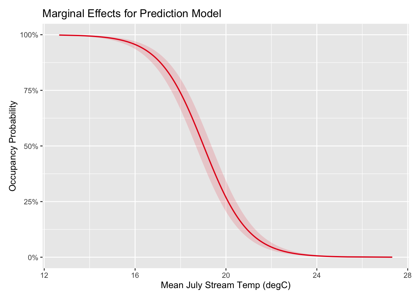
Figure 5.1: Marginal Effects Plot for Mean July Stream Temperature (Prediction Model)
The HUC8 random effect intercepts were also relatively similar to those from the initial calibration model.
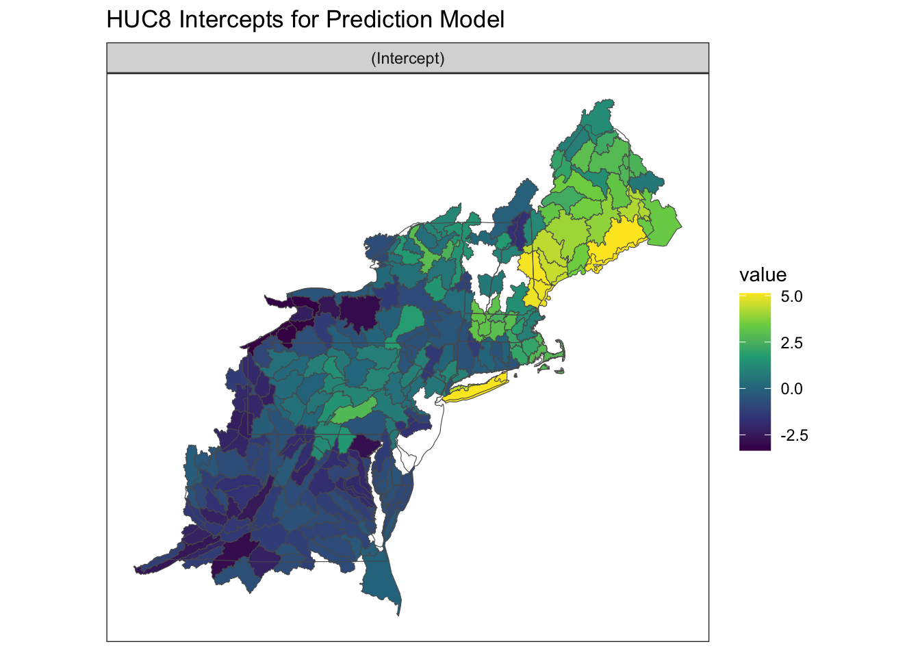
Figure 5.2: Random Effect Intercept by HUC8 Basin (Prediction Model)
The following output summarizes the prediction model’s accuracy and performance (see Calibration for explanation of this output).
Confusion Matrix and Statistics

          Reference
Prediction    0    1
         0 3334  888
         1 1295 7624

               Accuracy : 0.8339
                 95% CI : (0.8274, 0.8402)
    No Information Rate : 0.6477
    P-Value [Acc > NIR] : < 2.2e-16

                  Kappa : 0.6285

 Mcnemar's Test P-Value : < 2.2e-16

            Sensitivity : 0.8957
            Specificity : 0.7202
         Pos Pred Value : 0.8548
         Neg Pred Value : 0.7897
             Prevalence : 0.6477
         Detection Rate : 0.5802
   Detection Prevalence : 0.6787
      Balanced Accuracy : 0.8080

       'Positive' Class : 1
The following table compares the performance of the prediction model using all available data to that of the calibration and validation subsets (see Calibration and Validation). Overall, the full prediction model performs very similarly to the initial calibration model.
| Metric | Calibration | Validation | Full (Prediction) |
|---|---|---|---|
| Accuracy | 0.836 | 0.811 | 0.834 |
| Sensitivity | 0.899 | 0.840 | 0.896 |
| Specificity | 0.720 | 0.759 | 0.720 |
| Pos Pred Value | 0.856 | 0.862 | 0.855 |
| Neg Pred Value | 0.793 | 0.725 | 0.790 |
| Precision | 0.856 | 0.862 | 0.855 |
| Recall | 0.899 | 0.840 | 0.896 |
| F1 | 0.877 | 0.851 | 0.875 |
| Prevalence | 0.649 | 0.642 | 0.648 |
| Detection Rate | 0.583 | 0.539 | 0.580 |
| Detection Prevalence | 0.681 | 0.625 | 0.679 |
| Balanced Accuracy | 0.809 | 0.799 | 0.808 |
5.2 Prediction Metrics
Using the prediction model that was fitted to the full observation dataset, a series of occupancy metrics were computed for each catchment over the region (excluding those with cumulative drainage areas > 200 km2).
The prediction metrics include:
- Occupancy probability under historical conditions as well as air temperature increases of +2, +4, and +6 degC, which represents a series of simple climate change scenarios.
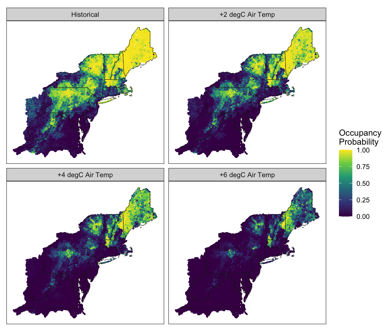
Figure 5.3: Predicted Occupancy Probabilities under Historical and Future Climate Change Scenarios
- The maximum increase in air temperature such that the predicted occupancy would be 30, 50, or 70%. These metrics indicate how resistant each catchment is to future climate change. Catchments with higher values can tolerate a larger increase in air temperature and still achieve each target occupancy probability.
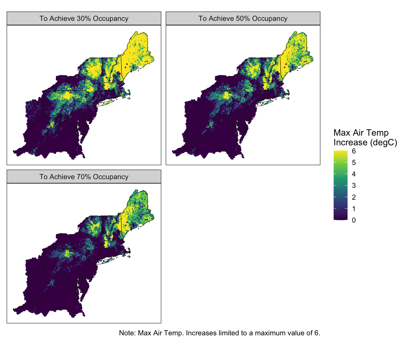
Figure 5.4: Predicted Max. Air Temperature Increases to Achieve Varying Occupancy Probabilities
A dataset containing the predicted values for these metrics can be downloaded in the Downloads section.